Patent Secrecy During WW2 and Future Citations

Image Processing and Computer Vision

Computer Vision, often abbreviated as CV, is defined as a field of study that seeks to develop techniques to help computers “see” and understand the content of digital images such as photographs and videos.

The problem of computer vision appears simple because it is trivially solved by people, even very young children. Nevertheless, it largely remains an unsolved problem based both on the limited understanding of biological vision and because of the complexity of visual perception in a dynamic and nearly infinitely varying physical world.

Desire for Computers to See

We require at least the same capabilities from computers in order to unlock our images and videos.

What Is Computer Vision?

Computer vision is a field of study focused on the problem of helping computers to see.

At an abstract level, the goal of computer vision problems is to use the observed image data to infer something about the world.

— Page 83, Computer Vision: Models, Learning, and Inference, 2012.

It is a multidisciplinary field that could broadly be called a subfield of artificial intelligence and machine learning, which may involve the use of specialized methods and make use of general learning algorithms.

Overview of the Relationship of Artificial Intelligence and Computer Vision

Computer vision as a field is an intellectual frontier. Like any frontier, it is exciting and disorganized, and there is often no reliable authority to appeal to. Many useful ideas have no theoretical grounding, and some theories are useless in practice; developed areas are widely scattered, and often one looks completely inaccessible from the other.

— Page xvii, Computer Vision: A Modern Approach, 2002.

The goal of computer vision is to understand the content of digital images. Typically, this involves developing methods that attempt to reproduce the capability of human vision.

Understanding the content of digital images may involve extracting a description from the image, which may be an object, a text description, a three-dimensional model, and so on.

Computer Vision and Image Processing

Computer vision is distinct from image processing.

Image processing is the process of creating a new image from an existing image, typically simplifying or enhancing the content in some way. It is a type of digital signal processing and is not concerned with understanding the content of an image.

A given computer vision system may require image processing to be applied to raw input, e.g. pre-processing images.

The goal of computer vision is to extract useful information from images. This has proved a surprisingly challenging task; it has occupied thousands of intelligent and creative minds over the last four decades, and despite this we are still far from being able to build a general-purpose “seeing machine.”

— Page 16, Computer Vision: Models, Learning, and Inference, 2012.

Studying biological vision requires an understanding of the perception organs like the eyes, as well as the interpretation of the perception within the brain. Much progress has been made, both in charting the process and in terms of discovering the tricks and shortcuts used by the system, although like any study that involves the brain, there is a long way to go.

Perceptual psychologists have spent decades trying to understand how the visual system works and, even though they can devise optical illusions to tease apart some of its principles, a complete solution to this puzzle remains elusive

— Page 3, Computer Vision: Algorithms and Applications, 2010.

Tasks in Computer Vision

omputer vision is at an extraordinary point in its development. The subject itself has been around since the 1960s, but only recently has it been possible to build useful computer systems using ideas from computer vision.

— Page xviii, Computer Vision: A Modern Approach, 2002.

t is a broad area of study with many specialized tasks and techniques, as well as specializations to target application domains.

Computer vision has a wide variety of applications, both old (e.g., mobile robot navigation, industrial inspection, and military intelligence) and new (e.g., human computer interaction, image retrieval in digital libraries, medical image analysis, and the realistic rendering of synthetic scenes in computer graphics).

— Page xvii, Computer Vision: A Modern Approach, 2002.

n this post, you discovered a gentle introduction to the field of computer vision.

Specifically, you learned:

• The goal of the field of computer vision and its distinctness from image processing.
• What makes the problem of computer vision challenging.
• Typical problems or tasks pursued in computer vision.

Many popular computer vision applications involve trying to recognize things in photographs; for example:

• Object Classification: What broad category of object is in this photograph?
• Object Identification: Which type of a given object is in this photograph?
• Object Verification: Is the object in the photograph?
• Object Detection: Where are the objects in the photograph?
• Object Landmark Detection: What are the key points for the object in the photograph?
• Object Segmentation: What pixels belong to the object in the image?
• Object Recognition: What objects are in this photograph and where are they?

Screenshots of ofx-kikko by Cyril Diagne

In the example below, one pass of erosion is applied to the image at left. This eliminates all of the isolated specks of noise:

Original image (left), after one pass of erosion (right)

By contrast, observe how dilation is used in the person-detecting pipeline below:

A complete image-processing pipeline, including

https://openframeworks.cc/ofBook/chapters/image_processing_computer_vision.html

Finding extreme points in contours with OpenCV

https://www.pyimagesearch.com/2016/04/11/finding-extreme-points-in-contours-with-opencv/

Figure 3: Finding extreme points along a contour with OpenCV plays a pivotal role in hand gesture recognition.

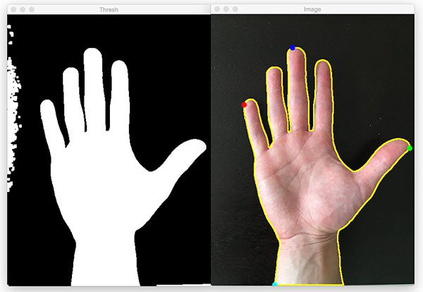
https://www.pyimagesearch.com/2016/04/11/finding-extreme-points-in-contours-with-opencv/

MATHLAB

Trace Boundaries of Objects in Images

https://www.mathworks.com/help/images/boundary-tracing-in-images.html

AUTOMATED ROCK SEGMENTATION FOR MARS EXPLORATION ROVER IMAGERY

Rock segmentation is important for the success of the Mars Exploration Rover mission and its scientific studies. In this paper, a framework for automated rock segmentation using texture-based image segmentation and edge-flow driven active contour is developed and implemented. Three schemes: wavelet-based local transform, multi-resolution histograms, and inter-scale decision fusion are combined and applied for texture-based image segmentation. The result is refined by active contour based on a level set method, which is propagated in the edge flow vector field. Test images taken by the panorama and navigation cameras on the rover Spirit at the Gusev Crater landing site are used in this study. This paper presents the theory, implementation, and the test results along with discussions on the performance of the proposed method.

Figure 2. Rock detection using texture-based segmentation [Input rock image (A), with K-means clustering (B), with interscale decision fusion clustering (C), and detected rock (D)]

igure 5. Edge flow and edge penalty function from rock image [Edge flow vector field (A), edge flows corresponding to the zoomed-in area (B), and computed edge penalty function (C)]

Figure 6. Rock boundary refinement by edge-flow driven active contours. [Yellow line denotes initial rock boundaries before refinement, red line is rock boundaries after refinement, and green lines is boundary propagation during refinement].

Figure 7a. Initial rock detection by texture-based segmentation

Figure 10. Detected rocks [NAVCAM image 1]

https://www.semanticscholar.org/paper/AUTOMATED-ROCK-SEGMENTATION-FOR-MARS-EXPLORATION-Song/aa7b43cef474de92dc12ff24beb90739a40581d1

Automating Science on Mars

Since 2016, NASA’s Curiosity Mars rover has had the ability to choose its own science targets using an onboard intelligent targeting system called AEGIS (for Automated Exploration for Gathering Increased Science). The AEGIS software can analyze images from on-board cameras, identify geological features of interest, prioritize and select among them, then immediately point the ChemCam instrument at selected targets to make scientific measurements.

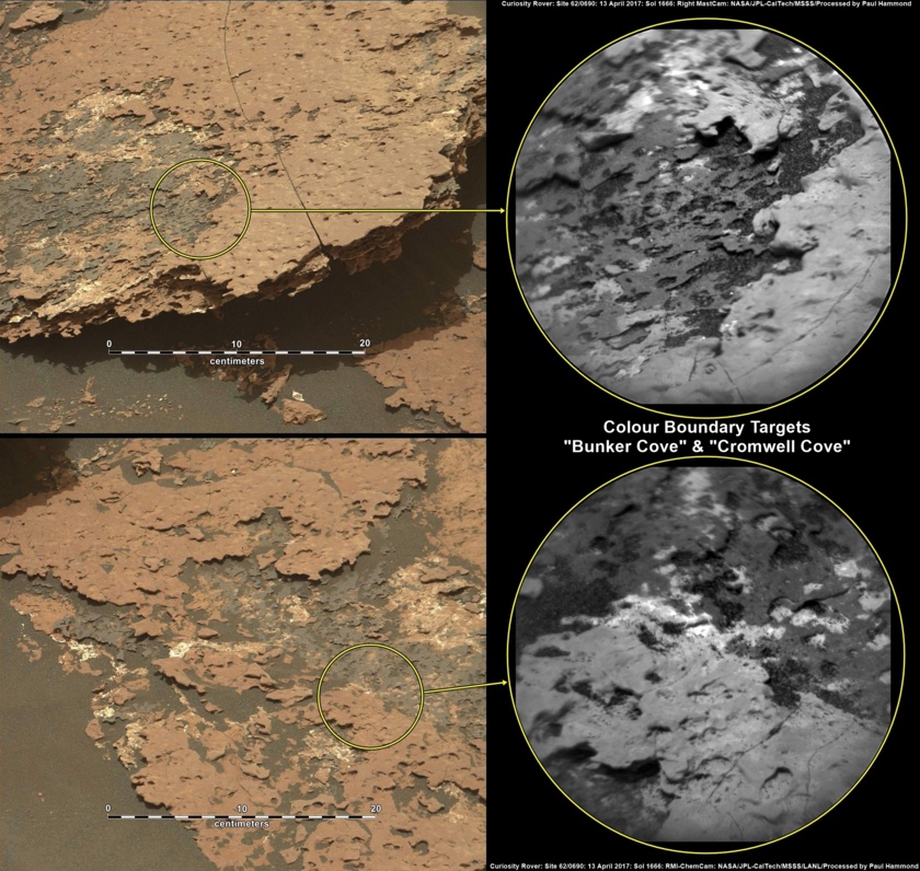
How it works

The AEGIS autonomous targeting process begins with taking a ‘source image’ – a photo with an onboard camera (either the NavCam or the RMI). AEGIS’ computer vision algorithms then analyze the image to find suitable targets for follow-up observations. On MER and MSL, AEGIS uses an algorithm called Rockster, which attempts to identify discrete objects by a combination of edge-detection, edge-segment grouping and morphological operations – in short, it finds sharp edges in the images, and attempts to group them into closed contours. Built originally to find float rocks on a sandy or gravelly background, Rockster has proved remarkably versatile at finding a variety of geological target types.

AN EXAMPLE OF ROCKSTER TARGET-FINDING

Using a particular scene profile, Rockster identified these targets in an MSL NavCam image on sol 1508.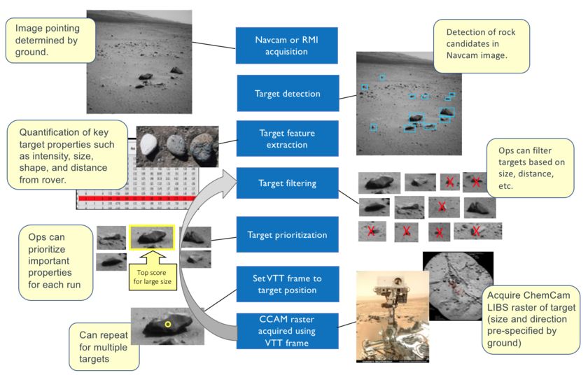

The autonomous targeting mode has been especially heavily used – more often than not, when Curiosity drives, it does AEGIS-guided ChemCam soon after. Running after most drives means that AEGIS has acquired ChemCam observations on over 130 targets (as of March 2018), and significantly increased the data rate from ChemCam. These are all targets which wouldn’t have been observed without onboard autonomy – they used the post-drive time when targeted observations aren’t possible because images of the new location haven’t yet been seen by the team on Earth.

The future

The success of AEGIS on MSL has led to its inclusion in NASA’s next Mars rover mission, to launch in 2020. That mission will have AEGIS available from the start of its surface operations, once again for targeting mast-mounted instruments. This will include SuperCam, the upgraded successor to ChemCam, with LIBS, RMI, but also Raman and infrared reflectance spectrometers.

The AEGIS team envisions other applications too. There are quite a number of places in the solar system where a robotic explorer can’t always wait around for Earthly operators to choose targets. Smarter robots with autonomous science capabilities will likely play an important role in exploring more challenging destinations, and mission designers and operators will learn to use these systems to share responsibility for decision-making with their distant robotic systems.

SCREENS

https://scikit-image.org/

https://scikit-image.org/docs/dev/auto_examples/color_exposure/plot_regional_maxima.html#sphx-glr-auto-examples-color-exposure-plot-regional-maxima-py

https://scikit-image.org/docs/dev/auto_examples/

....

Phyton  

 """
====================
Morphological Snakes
====================

*Morphological Snakes* [1]_ are a family of methods for image segmentation.
Their behavior is similar to that of active contours (for example, *Geodesic
Active Contours* [2]_ or *Active Contours without Edges* [3]_). However,
*Morphological Snakes* use morphological operators (such as dilation or
erosion) over a binary array instead of solving PDEs over a floating point
array, which is the standard approach for active contours. This makes
*Morphological Snakes* faster and numerically more stable than their
traditional counterpart.

There are two *Morphological Snakes* methods available in this implementation:
*Morphological Geodesic Active Contours* (**MorphGAC**, implemented in the
function ``morphological_geodesic_active_contour``) and *Morphological Active
Contours without Edges* (**MorphACWE**, implemented in the function
``morphological_chan_vese``).

**MorphGAC** is suitable for images with visible contours, even when these
contours might be noisy, cluttered, or partially unclear. It requires, however,
that the image is preprocessed to highlight the contours. This can be done
using the function ``inverse_gaussian_gradient``, although the user might want
to define their own version. The quality of the **MorphGAC** segmentation
depends greatly on this preprocessing step.

On the contrary, **MorphACWE** works well when the pixel values of the inside
and the outside regions of the object to segment have different averages.
Unlike **MorphGAC**, **MorphACWE** does not require that the contours of the
object are well defined, and it works over the original image without any
preceding processing. This makes **MorphACWE** easier to use and tune than
**MorphGAC**.

References
----------

.. [1] A Morphological Approach to Curvature-based Evolution of Curves and
       Surfaces, Pablo Márquez-Neila, Luis Baumela and Luis Álvarez. In IEEE
       Transactions on Pattern Analysis and Machine Intelligence (PAMI),
       2014, :DOI:`10.1109/TPAMI.2013.106`
.. [2] Geodesic Active Contours, Vicent Caselles, Ron Kimmel and Guillermo
       Sapiro. In International Journal of Computer Vision (IJCV), 1997,
       :DOI:`10.1023/A:1007979827043`
.. [3] Active Contours without Edges, Tony Chan and Luminita Vese. In IEEE
       Transactions on Image Processing, 2001, :DOI:`10.1109/83.902291`

"""

import numpy as np
import matplotlib.pyplot as plt
from skimage import data, img_as_float
from skimage.segmentation import (morphological_chan_vese,
                                  morphological_geodesic_active_contour,
                                  inverse_gaussian_gradient,
                                  checkerboard_level_set)


def store_evolution_in(lst):
    """Returns a callback function to store the evolution of the level sets in
    the given list.
    """

    def _store(x):
        lst.append(np.copy(x))

    return _store


# Morphological ACWE
image = img_as_float(data.camera())

# Initial level set
init_ls = checkerboard_level_set(image.shape, 6)
# List with intermediate results for plotting the evolution
evolution = []
callback = store_evolution_in(evolution)
ls = morphological_chan_vese(image, 35, init_level_set=init_ls, smoothing=3,
                             iter_callback=callback)

fig, axes = plt.subplots(2, 2, figsize=(8, 8))
ax = axes.flatten()

ax[0].imshow(image, cmap="gray")
ax[0].set_axis_off()
ax[0].contour(ls, [0.5], colors='r')
ax[0].set_title("Morphological ACWE segmentation", fontsize=12)

ax[1].imshow(ls, cmap="gray")
ax[1].set_axis_off()
contour = ax[1].contour(evolution[2], [0.5], colors='g')
contour.collections[0].set_label("Iteration 2")
contour = ax[1].contour(evolution[7], [0.5], colors='y')
contour.collections[0].set_label("Iteration 7")
contour = ax[1].contour(evolution[-1], [0.5], colors='r')
contour.collections[0].set_label("Iteration 35")
ax[1].legend(loc="upper right")
title = "Morphological ACWE evolution"
ax[1].set_title(title, fontsize=12)


# Morphological GAC
image = img_as_float(data.coins())
gimage = inverse_gaussian_gradient(image)

# Initial level set
init_ls = np.zeros(image.shape, dtype=np.int8)
init_ls[10:-10, 10:-10] = 1
# List with intermediate results for plotting the evolution
evolution = []
callback = store_evolution_in(evolution)
ls = morphological_geodesic_active_contour(gimage, 230, init_ls,
                                           smoothing=1, balloon=-1,
                                           threshold=0.69,
                                           iter_callback=callback)

ax[2].imshow(image, cmap="gray")
ax[2].set_axis_off()
ax[2].contour(ls, [0.5], colors='r')
ax[2].set_title("Morphological GAC segmentation", fontsize=12)

ax[3].imshow(ls, cmap="gray")
ax[3].set_axis_off()
contour = ax[3].contour(evolution[0], [0.5], colors='g')
contour.collections[0].set_label("Iteration 0")
contour = ax[3].contour(evolution[100], [0.5], colors='y')
contour.collections[0].set_label("Iteration 100")
contour = ax[3].contour(evolution[-1], [0.5], colors='r')
contour.collections[0].set_label("Iteration 230")
ax[3].legend(loc="upper right")
title = "Morphological GAC evolution"
ax[3].set_title(title, fontsize=12)

fig.tight_layout()
plt.show()